Common used random variables

In this post, I am going to summarize some common used random variables for future references.

Bernoulli Distribution

A Bernoulli distribution is the simplest discrete probability distribution, representing a single trial that has only two possible outcomes: success (usually denoted by 1) or failure (usually denoted by 0). $ T_t $ has one parameter $ p $, which represents the probability of success.

Mean and Variance

Binomial Distribution

A Binomial distribution represents the number of successes in a fixed number of independent Bernoulli trials, each with the same probability of success. The binomial distribution has parameters $(n, p)$ with $n$ as the number of trails and $p$ is the probability of success of one Bernoulli trail.

The PMF is:

Mean and Variance

Poisson Distribution

Poisson is a discrete probability distribution to express the probability of a given number of events occurring in a fixed interval of time (i.e. the number of tasks arriving in queuing systems). These events occur with a known mean rate $(\lambda)$ and independently of the time since the last event. The Poisson distribution deals with the number of occurrences in a fixed period of time, and the exponential distribution deals with the time between occurrences of successive events as time flows by continuously.

The probability mass function is:

The positive real number $\lambda$ is equal to the expected value, and the variance of $X$:

The Poisson distribution can be seen as a limit of the binomial distribution under certain conditions. This is known as the Poisson approximation to the binomial distribution.

The Poisson distribution is a good approximation to the binomial distribution when:

1. $n$ is large (the number of trials is large).
2. $p$ is small (the probability of success in each trial is small).
3. The product $np=\lambda$ is moderate (the expected number of successes remains constant).

Additivity: if $X_i \sim \rm{Poisson(\lambda_i)}$, for $i = 1, 2, \dots, n$, and the $X_i$ is independent, then

Poisson distribution as an approximation of Binomial distribution

As a rule of thumb, if $n \ge 100 $ and $np < 10$, the Poisson distribution (taking $\lambda = np$​​) can provide a very good approximation to the binomial distribution.

One important limit is used to prove the approximation:

To better see the connection between these two distributions, consider the binomial probability of seeing $x$ successes in $n$ trials, with the aforementioned probability of success, $p$, as shown below.

Let denote the expected value of the binomial distribution as $\lambda = np$, which means $p = \frac{\lambda}{n}$. Here $\lambda$ is also the arriving rate of success event of the approximated Poisson distribution.

The probability mass function can be written as follows:

Using the standard formula for the combinations of $n$ things taken $x$ at a time and some simple properties of exponents, we can further expand things to

Notice that there are exactly x𝑥 factors in the numerator of the first fraction. Let us swap denominators between the first and second fractions, splitting the$ $n^x$ all of the factors of the first fraction’s numerator.

Finally, applying the limit to $P(x)$ and keeping $x, \lambda$ Fiexed:

Exponential Distribution

For the continuous version of exponential distribution, the probability density function (PDF):

Here $\lambda$ > 0 is the parameter of the distribution, often called the rate parameter. The distribution is supported on the interval [0, $\infty$). If a random variable X has this distribution, we write $X \sim \rm{Exp}(\lambda)$.

The cumulative distribution function:

The CDF and PDF are not the actual probability. For continuous probability distribution, we only compute the probability of a given interval instead of one single point. Because the probability $P(a \le x \le b)$ is the integral of PDF values in the range of $[a, b]$ and the area under a single point is infinitesimally small. The CDF is the integral of PDF, we can simple compute the probability as:

where $F(x)$ is the CDF of $x$.

Property:

• Mean: $\frac{1}{\lambda}$
• Variance: $\frac{1}{\lambda^2}$​
• Memoryless: The exponential distribution and the geometric distribution are the only memoryless probability distributions.

Poisson Process

Let $\lambda > 0$ be fixed. The counting process ${N(t), t \in [0, \infty)}$ is called a Poisson Process with rate $\lambda$ if all the following conditions hold:

• $N(0) = 0$;
• $N(t)$​ has independent increments;
• The number of arrivals in any interval of length $\tau > 0$ has $\rm{Poisson}(\lambda \tau)$ distribution.

Note that from the above definition, we conclude that in a Poisson process, the distribution of the number of arrivals in any interval depends only on the length of the interval, and not on the exact location of the interval on the real line. Therefore the Poisson process has stationary increments.

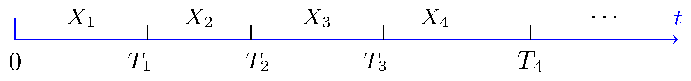
We denote $X_1$ as the interval of the first arrival, the $T_1$ is the time instant of first arrival.

If $N(t)$ is a Poisson process with rate $\lambda$, then the. interarrival times $X_1, X_2, \dots$ are independent and

$X$ is a memoryless random variable, that is

Thinking of the Poisson process, the memoryless property of the interarrival times is consistent with the independent increment property of the Poisson distribution. In some sense, both are implying that the number of arrivals in non-overlapping intervals are independent.

Since the arrival time can be derived by:

\(\begin{align} T_1 =X_1 \\ T_2 =X_1 + X_2 \\ T_3 =X_1 + X_2 + X_3 \end{align}\) More specifically, $T_n$ is the sum of $n$ independent $\rm{Exponential}(\lambda)$ random variables. Then $T_n \sim \rm{Gamma(n, \lambda)}$. Note that here $n \in \mathbb{N}$. The $\rm{Gamma(n, \lambda)}$​ is also called Erlang distribution, i.e, we can write

The PDF of $T_n$, for $n = 1, 2, 3, \dots$, is given by

and

Markov Chain

Given the past states $X_0, X_1, \dots, X_n-1$ and the current state $X_n$, a Markov chain is a stochastic process, where the conditional distribution of any future state $X_{n+1}$ is independent of the past states and depends solely on current state. The $P_{ij}$ represents the probability of the process transiting from state $i$ to $j$, and the one-step transition matrix is a 2D matrix containing all possible probability of states transition. The multiple step transition can be obtained by the Chapman-Kolmogorov Equations:

Two states $i$ and $j$ that are accessible to each other are called to communicate. For any state, the process can never change since once entered is an absorbing state. Two states that communicate with each other are said to be in the same class, each state class is separate with another one. The Markov chain is irreducible if there is only one class (i.e., all states communicate with each other).

Limiting Probabilities

For an irreducible ergodic Markov (one class) chain $\lim_{n \rightarrow \infty} P^n_{ij}$ exists and is independent of $i$. It shows the limiting probability that the process will be in state $j$ at time $n$, which equals to the long-run proportion of time that the process will be in state $j$.

Mean Time Spent in Transient States

Considering a finite state Markov chain with states in range $T={1, 2, \dots, t}$, the transition probabilities matrix is a $t \times t$ matrix $P_T$. We denote the identity matrix as $I$. For transient state $i, j$, let $s_{ij}$ denotes the expected number of time periods that the Markov chain is in state $j$, given it starts from state $i$. The matrix format for transient state times is $S$, we have:

For each element, we can also compute the transition probability $f_{ij}$ from state $i$ to state $j$:

Where $\delta_{ij}$ is the corresponding element in identity matrix.